Subscribe to The Thoughtful Leader newsletter to discover leadership insights to elevate your team's performance.

Have you ever come across the term ‘stack ranking’ before?

It can also be referred to as a vitality curve, forced ranking, or rank and yank.

This is a method of measuring employee performance and then ranking employees against each other, from best to worst.

It was a standard developed by Jack Welch as CEO of General Electric in order to separate workers into 3 categories:

Top performers (top 20%)
Vital workers (middle 70%)
Non-producers (bottom 10%)

Stack ranking template

There is no shortage of information out there about the origins of stack ranking and the pros or cons of using it. Unfortunately, not many resources exist detailing *how* to actually perform stack ranking.

Not to worry! Your search for answers is over.

Team ManageBetter has taken the time to create a simple to use template and guide to help you give stack ranking a try.

Download our free stack ranking template for Excel.

Checklist for stack ranking

Here is a checklist of the information and values you will need to use the stack ranking template.

⬜ Employee names or IDs

This is what (who) you will be ranking.

⬜ Performance criteria

What items are you using to measure employee performance? Is it their attendance level, number of projects completed, ability to work quickly?

⬜ Scale for rating criteria

You must be able to give a numerical rating to each performance criteria. Whether you score out of 100 or 10 (or some other range) is up to you and your system.

⬜ Weight of each criteria

Stack ranking assumes that certain criteria are more important than others. Think about your performance criteria and how they relate in importance. This will allow you to assign more weight to more important criteria.

Guide for stack ranking template

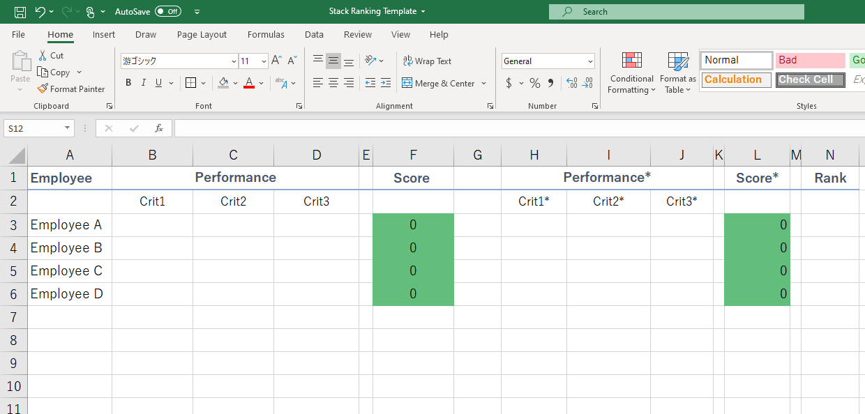
Step 1 - List employees

In the first column, list out your employees by name, employee ID or other identifier. This is the list you will want to rank based on performance variables.

Step 2 - List and score performance criteria

In the next columns, write the criteria on which you are basing your judgement of employee performance.

Include as many criteria items as necessary. In our example, we have three: Efficiency, Attendance, and Speed.

You need to assign a score to each of these categories based on the employee’s performance in that area.

The example above rates each on a scale of 1 to 10 (1 being worst performance, 10 being best performance).

Step 3 - Total scores of criteria

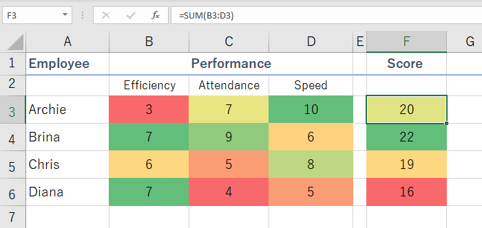
Create a column titled ‘Score’ next to the criteria categories. This will be the sum of an employee’s score in each criteria.

In the example, our equation for Archie’s ‘Score’ is =SUM(B3:D3).

Repeat the equation format for ‘Score’ (column F) for all other employees.

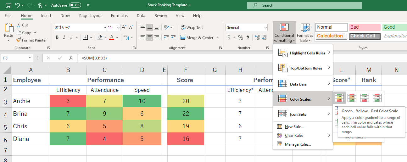
Step 4 - Apply color formatting

You can apply color formatting to criteria and score to give a visual representation of bad scores and good scores.

Use ‘conditional formatting’ in the upper navigation bar, and select ‘color scales’. Choose the first option so that low scores show red and high scores show green.

So is that it? Is Brina our top performer, in this example?

It’s a bit more complicated than that.

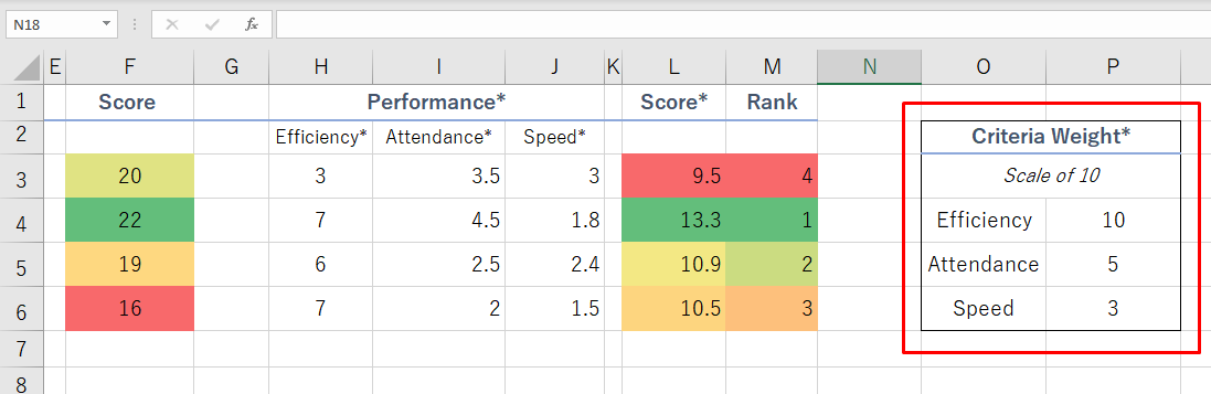
Step 5 - Decide criteria weights

Some performance criteria are going to be more important to employee success than others.

That is why we need to determine the weight that each criteria holds when calculating total score.

Score each criteria on a scale of importance. In the example, speed is least important, attendance is moderately important, and efficiency is highly important.

Note that multiple criteria can have the same level of importance. Simply remember to score them on the same scale.

Step 6 - Calculate weighted criteria scores and total scores

Now we need to calculate weighted scores for the criteria and total score. In the Excel template, a weighted item is denoted by an * asterisk.

Here, the equation for Archie’s weighted efficiency is =((B4*10)/10) .

That is his original efficiency score times the weight of efficiency (10) divided by the maximum potential weight (10).

Archie’s Attendance is calculated with =((C3*5)/10), and finally, speed is calculated with =((D3*3)/10).

The sum total of the criteria scores for Archie is =SUM(H3:J3).

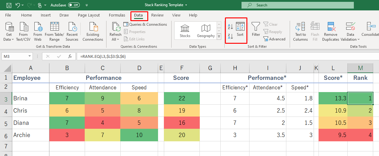
Step 7 - Rank the employees

Finally!

Now we can use Excel’s Rank function to rank the list of employees based on their weighted score totals.

Simply use the equation =RANK.EQ(L3,$L$3:$L$6) in cell M3

The first input in the equation is the employee’s weighted total score (L3) and the second input is the range of all employee weighted total scores ($L$3:$L$6). Be sure to hit F4 so the range becomes an absolute reference for all of the following rank function equations.

Lastly, go to the Data tab at the top and sort your data according to column M ‘Rank’ from lowest to highest. This will rank your employees in order from top performer to worst performer.

Our rank shows that Brina is the top performer, then Chris, Diana, and Archie.

Takeaways

As we can see above, stack ranking gives a clear and data-driven look at the performance of employees.

In the example, Archie appeared to be number 2 in the rank based on initial scores. But once the weight of each criteria was accounted for, Archie actually ended up ranking last. Despite his good performance in other areas, his poor performance in the most important criteria (efficiency) made him rank lower.

There may be times when two or more employees achieve exactly the same total weighted score (Column L). In these cases, the employees will be given the same rank.

It will be up to you to decide who ranks higher or lower.